
How to Calculate Pearson Correlation Coefficient by Hand (Step-by-Step Guide)
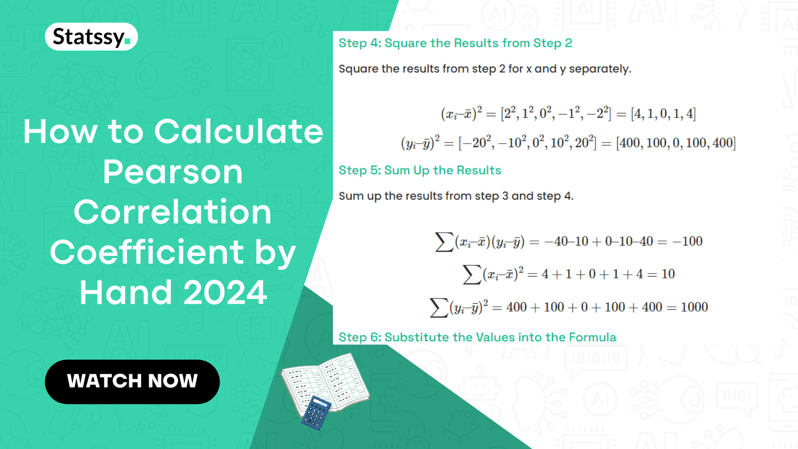
To calculate the Pearson correlation coefficient by hand, find the mean of x and y, subtract each mean from its own values to get the deviations, multiply and square those deviations, sum each column, then plug the three sums into the formula r = Σ(xᵢ – x̄)(yᵢ – ȳ) / √[Σ(xᵢ – x̄)² × Σ(yᵢ – ȳ)²].
How to calculate Pearson correlation coefficient by hand is one of the questions I get asked most often by dissertation students, even the ones who already run SPSS or R without any trouble. Software gives you a number in one click, but if you cannot explain where that number came from, an examiner will notice within the first two follow-up questions. I have spent 12 years guiding research students through exactly this problem, so this article shows you how to compute Pearson correlation manually, one column at a time. By the end, you will also know how to calculate Pearson correlation from scratch for your own dissertation dataset, not just for a textbook example.
What Is the Pearson Correlation Coefficient?
The Pearson correlation coefficient, denoted r, is a statistic that measures the strength and direction of the linear relationship between two continuous variables. It was named after the statistician Karl Pearson. Every value of r sits between -1 and +1, and that range alone tells you most of what you need to know before you look at the size of the number.
Range of r (-1 to +1) and What Each End Means
- r = +1: perfect positive correlation. As one variable rises, the other rises with it, in exact step.
- r = -1: perfect negative correlation. As one variable rises, the other falls, in exact step.
- r = 0: no linear correlation. The two variables move independently of each other.
Most real data falls somewhere between these three points. That is exactly why the third worked example further down matters more than the two textbook-perfect ones.
The Pearson Correlation Formula
r = Σ(xᵢ – x̄)(yᵢ – ȳ) / √[Σ(xᵢ – x̄)² × Σ(yᵢ – ȳ)²]
This is called the deviation-score formula, because each step works with how far a value sits from its own mean. The numerator is essentially the covariance between x and y, and the denominator scales it down using the standard deviation of each variable, which is just a formal way of describing how spread out the values are. There is also a raw-score version that skips the mean-subtraction step and works directly off Σx, Σy, Σxy, Σx² and Σy². I teach the deviation-score version first, because it makes the logic visible before you move to any shortcut.
How to Find Pearson Correlation Coefficient Step by Step
Here is the six-step method I use with every student, whether they are calculating Pearson r for a dissertation chapter or a stats class assignment. This step by step correlation coefficient calculation works the same way every time, no matter what x and y represent in your study.
- Find the mean of x and y. Add up all the x-values and divide by the count. Do the same for y. These two numbers are basic descriptive statistics, and every later step depends on them.
- Subtract the mean from each value. This gives you the deviation of each point from its own mean, for both x and y.
- Multiply the two deviations for each row. Multiply the x-deviation by the y-deviation, pair by pair.
- Square each deviation. Square the x-deviations and the y-deviations separately, in two more columns.
- Sum each column. Add up the products from step 3, and the two sets of squares from step 4.
- Plug the three sums into the formula. This gives you r.
A manual calculation of Pearson r with table is far less error-prone than trying to do it in your head. Building a table with columns for x, y, deviations, products and squares is the part most guides skip. This same method works for any sample size, you simply add more rows to the table, and past 15 to 20 pairs most students switch to software for the arithmetic but still use this table logic to sanity-check the output. I have written more on setting this up in my note on what tabular data actually is, worth reading if column layout confuses you.
Below is a full Pearson correlation coefficient worked example, done column by column, so you can check your own workings against a known answer before moving to messier numbers. Every Pearson correlation calculation with example numbers follows this same table structure, so once you have worked through one, you can repeat it for any dataset you are given.
Worked Example 1: Study Hours vs Test Scores (Perfect Positive Correlation)
| Student | Hours Studied (x) | Test Score (y) |
|---|---|---|
| 1 | 2 | 50 |
| 2 | 3 | 60 |
| 3 | 4 | 70 |
| 4 | 5 | 80 |
| 5 | 6 | 90 |
Mean of x = 4, mean of y = 70. Working through the six steps gives Σ(xᵢ-x̄)(yᵢ-ȳ) = 100, Σ(xᵢ-x̄)² = 10, and Σ(yᵢ-ȳ)² = 1000.
r = 100 / √(10 × 1000) = 100 / 100 = 1
Every extra hour studied adds exactly 10 points to the score, so the relationship is a perfect straight line. That is why r comes out to exactly 1.
Worked Example 2: Social Media Usage vs Test Scores (Perfect Negative Correlation)
Same students, same six steps, opposite direction this time.
| Student | Social Media Hours (x) | Test Score (y) |
|---|---|---|
| 1 | 2 | 90 |
| 2 | 3 | 80 |
| 3 | 4 | 70 |
| 4 | 5 | 60 |
| 5 | 6 | 50 |
Mean of x = 4, mean of y = 70. Σ(xᵢ-x̄)(yᵢ-ȳ) = -100, Σ(xᵢ-x̄)² = 10, and Σ(yᵢ-ȳ)² = 1000.
r = -100 / √(10 × 1000) = -100 / 100 = -1
Same method, opposite sign. This is Pearson r calculation for beginners at its cleanest, but I want to be honest with you. You will almost never see r = 1 or r = -1 in a real dissertation dataset.
Worked Example 3: A Realistic Dataset With an Imperfect Correlation
Most guides I have read online stop at the two examples above and leave you to figure out messy data on your own. That is a gap worth fixing here, because decimal figures and rounding are what you will actually face in a real chapter.
| Participant | Weekly Exercise (Hours) x | Sleep Quality Score y |
|---|---|---|
| 1 | 1.5 | 5.2 |
| 2 | 2.0 | 5.8 |
| 3 | 3.5 | 6.4 |
| 4 | 4.0 | 6.1 |
| 5 | 5.5 | 7.0 |
Mean of x = 3.3, mean of y = 6.1. Working through the same six steps: Σ(xᵢ-x̄)(yᵢ-ȳ) = 4.05, Σ(xᵢ-x̄)² = 10.30, and Σ(yᵢ-ȳ)² = 1.80.
r = 4.05 / √(10.30 × 1.80) = 4.05 / √18.54 ≈ 4.05 / 4.31 ≈ 0.94
Notice the rounding at every step. This is the part where students lose marks, not the formula itself. Round only at the final answer if your course allows it, and if intermediate rounding is required, keep at least three decimal places throughout so your final r does not drift.
It is also good practice to plot your data on a scatter plot before you trust any r value, since a strong-looking number can still hide a relationship that is not actually linear. The closer your points sit to the line of best fit running through them, the closer |r| will be to 1, whether positive or negative.
How to Interpret Your r Value
Once you calculate correlation coefficient without software, the next job is interpreting the number, and this is where a lot of published guides get sloppy. Since the sign only tells you the direction, here is how the size of r, ignoring plus or minus, is typically read:
| Size of r (Ignoring Sign) | Common Interpretation |
|---|---|
| 0.9 to 1.0 | Very strong |
| 0.7 to 0.89 | Strong |
| 0.5 to 0.69 | Moderate |
| 0.3 to 0.49 | Weak |
| 0.0 to 0.29 | Negligible |
Why “Strong vs Weak” Thresholds Vary by Field
Here is my honest opinion on most correlation guides you will find online. They present one interpretation scale as if it were a universal law, when it is not. A psychology paper might call r = 0.3 meaningful, while an engineering dataset would dismiss the same number as noise.
Cohen’s original benchmarks and the scale used in a peer-reviewed interpretation table built for clinical research do not fully agree with each other, sometimes by a full interpretation band for the same r value. Always check what threshold your own field or supervisor expects before writing “strong correlation” in your results chapter.
For a dissertation, reporting r alone is rarely enough. Most supervisors also want a significance test, meaning a p-value, and ideally a confidence interval around r, to show the result is not just a fluke of your sample size. In practice, this test converts your r and sample size into a t-statistic, and a p-value below 0.05 tells you the correlation is unlikely to have arisen by chance alone. A confidence interval then gives you a plausible range for the true population r, rather than treating your single sample estimate as exact.
Correlation Does Not Imply Causation
A high r value tells you two variables move together. It does not tell you that one causes the other. I have reviewed dissertation drafts where a student wrote “increased exercise causes better sleep” off a correlation table alone, and that line gets flagged in almost every viva I have sat through.
If you want to argue causation, you need an experimental design or additional statistical controls, not just a correlation coefficient. This is also where correlation work naturally leads into linear regression analysis later in a project.
Pearson vs Spearman: When to Use Which
Pearson’s r assumes your data is continuous, roughly normally distributed, and linearly related, with no serious outliers. If your normality assumption feels shaky, my guide on the Shapiro-Wilk test for normality will help you check that before you commit to Pearson.
When your data is ordinal, has outliers, or the relationship looks curved rather than straight, Spearman’s rank correlation is the safer choice, and Kendall’s tau is a close cousin often preferred for very small samples or a lot of tied ranks. I have laid out the full decision process in Pearson vs Spearman correlation: which one to use, including how to justify your choice to a supervisor.
Calculating Pearson r With Software (a Quick Signpost)
Once you have done this by hand two or three times and trust that you understand it, move to software for anything beyond a handful of data points. Excel’s CORREL function, Google Sheets, SPSS, and Python’s pandas or scipy libraries all compute r instantly. If several variables are involved, software can also build a full correlation matrix in seconds, something nobody would want to attempt by hand. If you are new to SPSS specifically, my SPSS data analysis tutoring page covers where this function sits inside the menus.
One thing I disagree with in several popular stats guides: a few tell readers that calculating Pearson correlation coefficient by hand is “hardly practical.” They push straight to software and skip the manual method entirely. I understand the instinct, but for a dissertation defence, being able to work through Pearson’s r by hand and explain each step out loud is what separates a student who understands their own analysis from one who is only reading numbers off a screen. It is the same reason I always tell students to verify any AI-generated statistics line by line rather than pasting them straight into a results chapter.
A Short Case Study From My Own Practice
A management student I once worked with had run her correlation analysis in SPSS correctly, but during her mock viva she could not explain what a moderate positive r actually meant beyond “it’s positive.” We sat down and recalculated a small subset of her data by hand, column by column. Within twenty minutes she could explain the deviation, the product, and the squared terms without looking at her notes.
Her actual viva went smoothly, and the software was never the problem. The gap was understanding.
Practice Problem (Your Free Worksheet)
Use this table as a Pearson correlation coefficient hand calculation worksheet. Try it yourself before checking the answer.
| Participant | Study Hours x | Score y |
|---|---|---|
| 1 | 1 | 55 |
| 2 | 2 | 58 |
| 3 | 3 | 65 |
| 4 | 4 | 63 |
| 5 | 5 | 70 |
Work through all six steps on paper. Mean of x = 3, mean of y = 62.2. If your Σ(xᵢ-x̄)(yᵢ-ȳ), Σ(xᵢ-x̄)² and Σ(yᵢ-ȳ)² come out to 35.0, 10 and 138.8, you are on the right track, and your final r should land at approximately 0.94.
These kinds of Pearson correlation coefficient practice problems are exactly what I set for students before they attempt their own dissertation dataset. Do two or three of these and the formula stops feeling abstract.
FAQ
What’s the difference between Pearson and Spearman correlation?
Pearson measures a straight-line relationship between two continuous variables. Spearman measures a monotonic relationship using ranked values, and handles ordinal data or outliers better. See the full comparison in u003ca href=u0022https://statssy.com/pearson-vs-spearman-correlation-which-one-to-use/u0022u003ePearson vs Spearman correlationu003c/au003e.
How do you calculate Pearson correlation in Excel?
Use the formula =CORREL(array1, array2), selecting your x-values and y-values as the two arrays. Excel returns r instantly, though I still recommend calculating it by hand at least once so you understand what the function is doing.
What are the assumptions of Pearson correlation?
Both variables should be continuous, roughly normally distributed, linearly related, and free of major outliers, with each pair of observations independent of the others. Checking normality first, using a formal normality test, is good practice before you report Pearson’s r.
What’s the minimum sample size for Pearson’s r?
There is no fixed legal minimum, but most methodology textbooks suggest at least 20 to 30 pairs for a stable, reportable correlation. Smaller samples can still produce a valid r, but the result becomes more sensitive to a single outlier.
u003cstrongu003eCan Pearson’s r be negative?u003c/strongu003e
Yes. A negative r simply means the two variables move in opposite directions, one rises as the other falls. It carries the same statistical validity as a positive r of the same size.
u003cstrongu003eWhat is r² and how is it different from r?u003c/strongu003e
r² is the coefficient of determination, found by squaring r. It tells you the proportion of variance in one variable that is statistically explained by the other, expressed as a percentage. An r of 0.8 gives an r² of 0.64, meaning 64% of the variance is shared between the two variables.
How do you test whether a Pearson correlation is statistically significant?
You convert your r value and sample size into a t-statistic and compare it against a critical value, or simply check the resulting p-value. A p-value below 0.05 generally means the correlation is unlikely to be due to chance, though a large sample can make even a weak r look statistically significant.
u003cstrongu003eWhat is the difference between correlation and covariance?u003c/strongu003e
Covariance tells you whether two variables move in the same or opposite direction, but its size depends on the units you measured them in. Pearson’s r is covariance divided by the standard deviations of both variables, which standardises it to a fixed -1 to +1 scale you can compare across studies.
If your dissertation analysis goes beyond a simple correlation table, or you want someone to check your workings before submission, my statistical consulting service is built exactly for that.
Author: Siddharth Gupta, MBA (Finance) and M.Tech, Director and Lead Engineer at IntalliaTech24, with 12+ years in analytics consulting and dissertation statistics guidance across R, Python, SPSS, Stata and Power BI. Connect on LinkedIn