
What are dt qt pt rt in R for Marketing Analytics
📑 Table of Contents
- → How I used Student t distribution to evaluate campaign performance
- → Why Student t distribution matters in marketing analytics
- → Marketing analytics scenario I worked on
- → Using dt in R to understand distribution shape
- → Using pt in R to calculate probability of campaign uplift
- → Using qt in R to build confidence intervals
- → Frequently Asked Questions
In marketing analytics, we rarely get perfect data.
Most of the time, we work with small samples, short campaign windows, and noisy customer behaviour.
How I used Student t distribution to evaluate campaign performance with limited data
In marketing analytics, we rarely get perfect data.
Most of the time, we work with small samples, short campaign windows, and noisy customer behaviour.
Early in my consulting work with a consumer internet business, I realised that normal distribution assumptions break down when sample sizes are small.
Why Student t distribution matters in marketing analytics
In many marketing problems, we try to estimate an average metric.
Conversion rate, daily revenue per user, average order value, email click rate.
The challenge is that campaigns often run for a short duration. Sample sizes remain small and population variance stays unknown.
In such situations, assuming a normal distribution leads to overconfidence.
Student t distribution corrects this by accounting for additional uncertainty.
💡 Key Insight
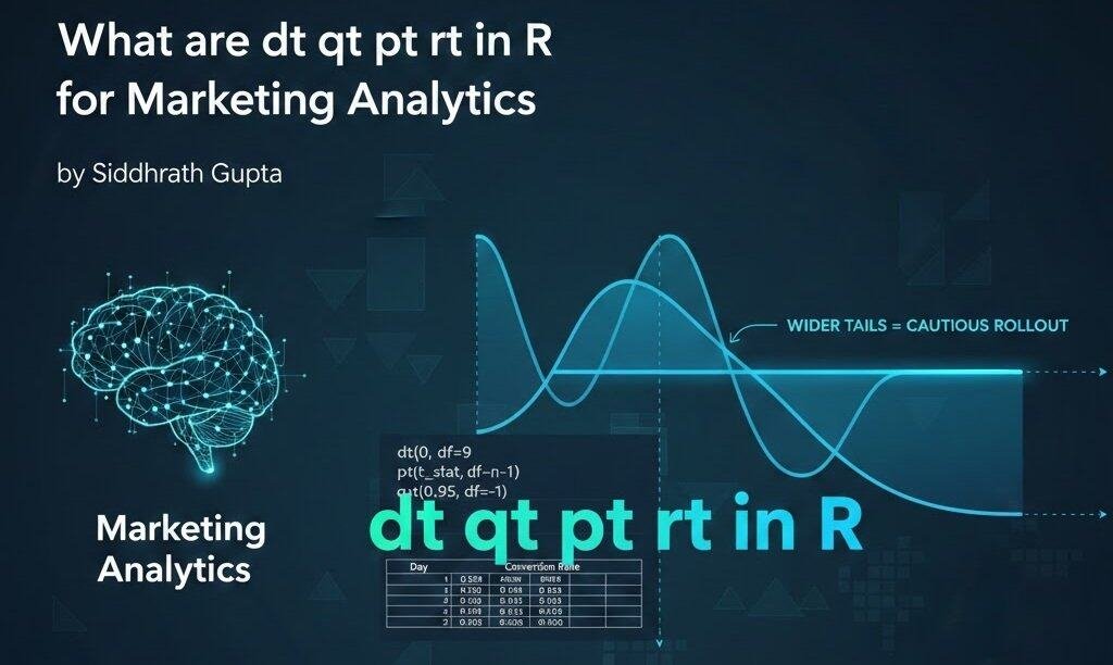
Student t distribution produces wider tails, which means extreme outcomes remain more likely than what normal distribution suggests. This prevents false confidence in small-sample marketing decisions.
From a business point of view, this prevents false confidence and bad rollout decisions.
The wider curve you see here is exactly what protects decision makers from aggressive conclusions based on limited data.


Marketing analytics scenario I worked on
The client was an online subscription based education platform.
They launched a new paid ad creative and wanted to know whether it genuinely improved daily conversion rate or whether the improvement was random.
The campaign ran for 10 days. Each day we tracked conversion rate from paid traffic.
This is realistic marketing data. Small sample, daily fluctuations, and pressure to decide quickly.
Hypothetical dataset similar to what I received
| Day | Conversion Rate |
|---|---|
| 1 | 0.028 |
| 2 | 0.031 |
| 3 | 0.030 |
| 4 | 0.027 |
| 5 | 0.032 |
| 6 | 0.029 |
| 7 | 0.033 |
| 8 | 0.030 |
| 9 | 0.031 |
The question was simple.
Is the average conversion rate truly higher than the historical benchmark of 2.8 percent.
Using dt in R to understand distribution shape of campaign performance
Before calculating probabilities, I like to understand how uncertain my estimate really is. This is where dt helps conceptually.
The dt function gives the height of the Student t probability density at a given value.
In simple words, it tells us how likely a particular t value is, given our sample size.
In this campaign, we had 10 observations. Degrees of freedom become 9.
dt(0, df = 9)
I do not use dt to answer business questions directly.
I use it to explain uncertainty to stakeholders.
When I plot the density using observed t values derived from real data points, the message becomes clear.
With small samples, the distribution stays wide.
That means we should expect volatility and avoid aggressive conclusions.
🎯 Practical Impact
Showing the marketing head this wide distribution curve helped them accept a cautious rollout plan instead of aggressive scaling.
This explanation alone helped the marketing head accept a cautious rollout plan.
Using pt in R to calculate probability of campaign uplift
pt is the function I use most in client work.
Conceptually, pt returns the probability that a random value from a Student t distribution is less than a given value.
In marketing terms, it helps answer probability style questions.
First, I compute the sample mean and standard deviation.
conv <- c(0.028,0.031,0.030,0.027,0.032,0.029,0.033,0.030,0.031,0.029)
xbar <- mean(conv)
s <- sd(conv)
n <- length(conv)
Then I calculate the t statistic comparing it with the historical benchmark.
benchmark <- 0.028
t_stat <- (xbar - benchmark) / (s / sqrt(n))
Now comes pt.
pt(t_stat, df = n - 1)
This value gives me the probability that the campaign performs better than the benchmark, considering uncertainty.
When I explain this to marketing teams, I say this.
This number tells us how confident we should feel that the improvement is real and not just random noise.
Using qt in R to build confidence intervals marketers understand
Decision makers rarely like yes or no answers. They prefer ranges.
qt helps find the cutoff points of the Student t distribution. These cutoffs allow us to build confidence intervals.
Frequently Asked Questions
❓ What is Student t distribution and why use it in marketing analytics?
Student t distribution accounts for uncertainty in small sample sizes. In marketing analytics, campaigns often run for short durations with limited data (typically 7-30 days). The t distribution produces wider tails than normal distribution, meaning extreme outcomes are more likely. This prevents false confidence and bad rollout decisions based on small samples. When sample sizes are small and population variance is unknown, using normal distribution leads to overconfidence in results.
❓ What does the dt function do in R?
The dt function in R gives the probability density (height) of the Student t distribution at a given value. It helps visualize and understand how uncertain your estimate is by showing the distribution shape. Syntax: dt(x, df) where x is the t-value and df is degrees of freedom (sample size - 1). Use dt to explain uncertainty to stakeholders rather than answer business questions directly. When plotted, it shows that with small samples, the distribution stays wide, indicating expected volatility.
❓ How do I use pt function in R for marketing decisions?
The pt function returns the cumulative probability that a value from Student t distribution is less than a given value. For marketing analysis: First, calculate the t-statistic using (sample_mean - benchmark) / (standard_deviation / sqrt(sample_size)). Then use pt(t_stat, df = n-1) to get the probability that campaign performance is better than the benchmark. This number tells you how confident you should feel that the improvement is real and not random noise, accounting for small sample uncertainty.
❓ What is qt function used for in R?
The qt function finds the critical values (cutoff points) of the Student t distribution, which are essential for building confidence intervals. Decision makers rarely want yes/no answers—they prefer ranges. qt helps provide these ranges. For example, qt(0.975, df=9) gives the t-value for a 95% confidence interval. Use it to construct intervals that communicate uncertainty in a way marketers understand, showing the range where the true campaign performance likely falls.
❓ When should I use Student t distribution instead of normal distribution?
Use Student t distribution when: (1) Sample size is small (typically n < 30), (2) Population variance is unknown, (3) You need to account for additional uncertainty from limited data. This is common in marketing with short campaign windows (7-14 days), daily conversion rate tracking, limited A/B test traffic, or pilot program evaluation. As sample size increases beyond 30, the t distribution converges to normal distribution, so the distinction becomes less important.
❓ What's the difference between dt, pt, qt, and rt in R?
These are the four core Student t distribution functions in R: dt (density) - gives probability density at a point, used for understanding distribution shape; pt (probability) - gives cumulative probability, used for hypothesis testing and calculating p-values; qt (quantile) - gives critical values for confidence intervals; rt (random) - generates random values from t distribution, used for simulation and Monte Carlo analysis. Each serves a specific purpose in marketing analytics statistical workflow.
❓ How many data points do I need to use Student t distribution?
You can use Student t distribution with as few as 2 data points (though more is better). It's specifically designed for small samples. Common marketing scenarios: 7-10 days of daily conversion rates, 10-20 days of campaign data, or 15-30 customer responses in a pilot test. The beauty of t distribution is that it properly accounts for uncertainty when you have limited data. With 30+ observations, you can use either t or normal distribution as they converge.
📊 Work With Me
Need help with marketing analytics, pricing strategy, or data-driven decision making? I work with founders and leadership teams to turn data into actionable insights.
Remote consulting engagements • Full-time roles • Power BI, R, SQL, Tableau
👤 About the Author
Siddharth Gupta is an Analytics Consultant specializing in pricing strategy, growth analytics, and data-driven decision making. Since 2017, he has delivered analytics engagements across SaaS, D2C, logistics, education, and professional services sectors.
His work focuses on turning complex data into decision-ready insights that support revenue growth, cost control, and performance improvement. He works with Power BI, Tableau, Excel, R, and SQL to create actionable business intelligence.