SPSS Data Cleaning: How One Overlooked Boxplot Nearly Sank a DNP Dissertation Defence

SPSS data cleaning is the step almost every graduate student treats as a formality, a quick missing-value check before the “real” analysis begins. I have been guiding dissertation and DNP students through their statistics for twelve years now, and in my experience, this is the single most skipped step in the entire process.

If you are searching for dissertation data cleaning SPSS help because your own defence date is closing in, the case below is probably close to your situation. A student I worked with, four months out from her defence, found out the hard way what skipping this step costs.

Her project was a retrospective chart review, one of the more common secondary-data designs in DNP work, testing whether a nurse-led hypertension programme lowered systolic blood pressure. Two hundred and twelve patients, split evenly into an intervention group and a matched comparison group. She had already run her independent samples t-test, and the result was significant.

Her advisor was pleased. Then a committee member asked one question that unravelled the whole analysis: “Did you check for outliers before you ran that?” She had not. This article walks through what we found, what we fixed, and why the fix mattered more than the original result.

What Counts as an Outlier in SPSS (Not Just “Weird Numbers”)

An outlier in SPSS is a data point that falls far enough from the rest of your distribution that it is unlikely to belong to the same population, usually flagged when it sits more than 1.5 box-lengths (mild) or 3 box-lengths (extreme) beyond the edges of a boxplot. That is the working definition inside SPSS’s own Explore procedure, and it is worth memorising because most students think “outlier” simply means anything that looks odd to the eye.

In practice, when you look up how to run this procedure, most guides explain the syntax and stop there. They tell you how to produce the boxplot and say nothing about what to do once you are staring at eleven extreme values with a defence date approaching. That gap between “here is the output” and “here is what you do next” is exactly where students get stuck, and it is the gap this article tries to close.

How to Run a Boxplot and Stem-and-Leaf Check (EXAMINE Syntax)

Before running any t-test, run this in SPSS syntax:

EXAMINE VARIABLES=change_sbp
  /PLOT BOXPLOT STEMLEAF HISTOGRAM
  /COMPARE GROUPS
  /STATISTICS DESCRIPTIVES EXTREME
  /CINTERVAL 95
  /MISSING LISTWISE
  /NOTOTAL.

This single block gives you the boxplot, the stem-and-leaf plot, and a list of the most extreme cases with their case ID numbers. If you have not opened the Explore menu before writing your results chapter, this is usually why your committee keeps circling back to it.

Reading SPSS Boxplot Outliers: Mild vs Extreme

SPSS boxplot outliers interpretation comes down to two categories:

1. Mild outliers sit between 1.5 and 3 box-lengths from the edge of the box, marked with a circle. Usually genuine, unusual scores worth a second look, not automatically a problem.
2. Extreme outliers sit beyond 3 box-lengths, marked with an asterisk. These deserve verification against source data before you trust them in any analysis.

The Real Case: Impossible Blood Pressure Values in a Hypertension Study

When I asked for the raw data, the syntax, and the descriptive output, the problem showed up within twenty minutes. The change score variable had a mean of minus 9.15 mmHg, a standard deviation of 18.4, and a range running from minus 187 to plus 112 mmHg.

A systolic blood pressure change of minus 187 mmHg is not something a human body produces. Neither is plus 112. These were not genuine extreme responders. They were errors sitting inside a dataset that had already been analysed and written up.

What the Descriptive Statistics Missed

The boxplot showed eleven extreme outliers, points sitting well beyond three box-lengths from the box edge. The stem-and-leaf plot confirmed a long left tail with a handful of implausible values dragging the mean around. None of this shows up in a plain independent samples t-test output. You have to go looking for it.

Verifying Outliers Against Source Data

We went back to the original chart data for all eleven cases. Six were straightforward data entry errors, 187 typed instead of 87, with the sign flipped by the change calculation. Three were unit conversion mistakes carried over from an earlier recording format. Two could not be verified against any source document at all.

SPSS Data Cleaning: Four Ways to Handle an Outlier (and the One That Gets Students in Trouble)

Once you find an outlier, you have exactly four honest options.

1. Correct it, if you can verify the true value against the original source.
2. Remove it, if it is a confirmed error you cannot correct, and document the removal with the case ID and reason.
3. Winsorise it, replacing the extreme value with a less extreme percentile value from the same distribution.
4. Keep it and use an outlier-resistant test instead of the standard t-test, such as a Mann-Whitney U.

The option that is not on this list, and the one I see students reach for most under deadline pressure, is quietly deleting anything that “looks wrong” with no verification and no record. That is not dissertation data cleaning SPSS work. That is data manipulation, and a committee that catches it will not just ask you to redo the analysis.

Correct, Remove, Winsorise, or Use an Outlier-Resistant Test

In this case, we corrected the six entry errors, fixed the three conversion errors, and removed the two unverifiable cases. The corrected dataset had a mean change of minus 8.2 mmHg, a standard deviation of 11.7, and a range from minus 52 to plus 38. That range is physiologically believable. The earlier one was not.

For anyone running this analysis themselves, a Wilcoxon signed-rank calculator or a Shapiro-Wilk test calculator is a fast way to sanity-check a corrected dataset before you commit to a test.

Building a Data Cleaning Log Your Committee Will Accept

We logged every one of the eleven cases by ID, the value found, the corrected or removed value, and the source used to verify it. Her committee chair signed off on this log without objection at the defence. This is the part most SPSS guides never mention, because most are written for readers who are not actually defending anything to a committee.

If you want a starting point, a simple four-column table works: case ID, original value, corrected or removed value, and verification source. I walk students through building this exact log as part of SPSS data cleaning support sessions, and it usually takes under ten minutes to adapt to a new dataset.

Paired Samples t-Test in SPSS vs Independent Samples: Which One Is Yours?

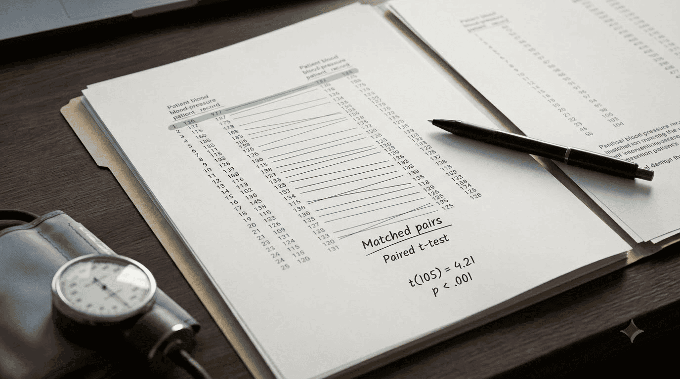
Here is where the second, bigger problem showed up. Her design was described as a “matched comparison group.” Each intervention patient had been matched one-to-one to a comparison patient on age, sex, and baseline blood pressure. That is a paired design.

She had analysed it as two independent groups instead. Running a paired samples t-test in SPSS on data that is actually matched pairs is not a stylistic choice: it changes the answer, because an independent samples test throws away the matching information and treats every observation as unrelated to every other one.

A peer-reviewed review of statistical practice in medical research papers found that misapplying independent-samples tests to matched-pairs data is a persistent error across published studies, not a rare one. What a journal review like that will not give you is a practical way out for a student sitting alone with SPSS four months before a defence. That practical fix is what the rest of this section covers, alongside a closer look at paired versus repeated-measures designs if your project involves more than two time points.

How to Tell If Your Comparison Groups Are Actually Matched

Ask yourself one question: was each participant in Group A deliberately linked to one specific participant in Group B before data collection began, on variables like age, sex, or baseline score? If yes, you have paired data, whatever your methods chapter happens to call it.

SPSS Syntax for a Paired Samples t-Test

Once the data was restructured so each row held one matched pair, the syntax was straightforward:

T-TEST PAIRS=change_intervention WITH change_comparison (PAIRED)
  /CRITERIA=CI(.95)
  /MISSING=ANALYSIS.

The paired result: mean difference of minus 6.8 mmHg, t(105) = 4.21, p < .001. The effect was larger and more precisely estimated than her original independent-samples version, because pairing removes between-pair variability from the error term. Her original analysis had understated her own intervention’s real effect.

Checking Assumptions Before You Trust the t-Test

Fixing the outliers and the test type does not finish the job. You still need to confirm a t-test is the right tool at all, and this is where a Shapiro-Wilk normality guide becomes useful for your own dataset, not just this case.

Shapiro-Wilk, Q-Q Plots and Levene’s Test in SPSS

As a general rule, a Shapiro-Wilk p-value below .05 signals a meaningful departure from normality, while a value above .05 means normality is a reasonable assumption. In this case, Shapiro-Wilk came back significant for both groups, p < .001 for intervention and p = .003 for comparison, but the Q-Q plots showed only mild departure in the tails.

Levene’s test works the same way in reverse: a p-value below .05 means your two groups’ variances differ enough to matter, above .05 means the equal-variance assumption holds. Here, Levene’s test was not significant, p = .41, so that assumption was fine.

When to Add a Mann-Whitney U as a Cross-Check

With 106 patients per group, mild non-normality is not fatal to a t-test, but I still had her run a Mann-Whitney U test as a cross-check. It came back consistent, U = 4,118, p < .001. When your parametric and non-parametric results agree, that agreement is worth a sentence in your results chapter, because it heads off exactly the kind of question that started this whole review.

Reporting the Correct Effect Size for a Paired Design

Her draft reported Cohen’s d for an independent samples comparison, calculated at 0.53, a medium effect. That is the wrong effect size formula for a paired design.

Cohen’s d vs Cohen’s d_z, Why They Differ

For paired data, the correct effect size is Cohen’s d_z, the mean difference divided by the standard deviation of the difference scores, not the pooled standard deviation used for independent groups. Standard effect-size reporting practice requires the formula to match the test structure, not just the test name; it is one of the first things I flag when a student sends me statistics to review. Recalculated properly using an effect size calculator, hers came out to 0.41, still small to medium, but built on a different denominator. I had her report both values with a short note on which one applies to her design, since a sharp committee member will ask if only one number appears without explanation.

Statistics Help for DNP and Nursing Dissertations: When to Get a Second Opinion

Your advisor approving your analysis is not the same as your analysis being correct. Advisors are experts in your clinical field, not always in SPSS syntax, and that gap is exactly where cases like this one slip through.

I have seen the same pattern show up outside health research too, often in a similar shape. In one MBA dissertation using structural equation modelling for an employee engagement study, a handful of Likert-scale entries had been coded outside the valid range and were being treated as legitimate scores by the software for months.

A simple FREQUENCIES run in week one would have caught it. Instead it surfaced only once model fit stayed stubbornly weak, and once the miscoded entries were cleaned, fit improved to a comfortably acceptable range.

Neither of these students was careless. Both were simply never taught that data cleaning means more than checking for blanks. This is exactly the kind of statistics help for DNP project work I get asked to do most, and it rarely means redoing the whole study or spending heavily on a full re-analysis. Often it means a focused review of five things: outliers, test selection, assumptions, matching, and effect size, which is usually a matter of hours, not weeks.

If you are unsure whether your own project needs a second pair of eyes before defence, this guide on how to know if you need a dissertation expert is a fair starting point, and it does not assume the answer is always yes. If you decide it does, how to find a dissertation writing mentor covers what to look for before you commit to anyone.

SPSS help for a nursing dissertation does not need to mean redoing your whole study.

The Takeaway

Finding an error in your data late does not make your study invalid. It means the study is being checked properly, which is what a defence is supposed to test in the first place. The t-test here was significant before the corrections and after them. Her intervention genuinely worked.

But she had been four months away from defending an analysis built on eleven impossible values, the wrong test structure, and the wrong effect size formula. Any one of those three, caught at the defence table instead of before it, could have meant a delayed defence rather than a passed one.

SPSS will run a t-test on data containing a value of minus 187 mmHg without complaint. It will give you a p-value. It will not stop you from publishing a physiologically impossible number in your results chapter. The boxplot sits inside the Explore menu the whole time, and in twelve years of this work, I have met very few students who opened it before someone made them.

FAQ