
12 Stata Logistic Regression Interpretation Mistakes Students Make
By Siddharth Gupta | Last updated: 4 November 2026 | Reading time: about 12 minutes
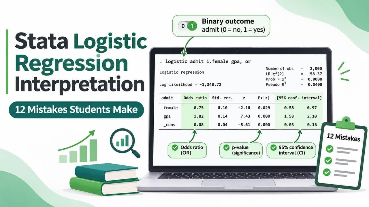
Stata logistic regression interpretation goes wrong in the same places, year after year. In my 12 years of dissertation work, I have seen students run the model correctly and then write a results paragraph that loses marks.
The code is rarely the problem. The sentence after the code is.
Below are the 12 mistakes I see most, with logit, logistic and logit, or examples and wording you can adapt for your own results chapter. I cite StataCorp’s documentation and the papers listed at the end, and I say where I disagree with them.
What is Stata logistic regression interpretation? It means reading the output of
logitorlogisticand explaining how each predictor changes the odds of a binary outcome, holding the other predictors constant. Effects are reported as log-odds coefficients (logit) or odds ratios (logisticorlogit, or), always with a 95% confidence interval.
The 12 Stata Logistic Regression Interpretation Mistakes at a Glance
- Confusing log-odds with odds ratios
- Reading odds ratios as risk ratios
- Getting odds ratios below 1 backwards
- Ignoring confidence intervals
- Using the wrong reference category
- Coding the outcome wrongly
- Misreading odds ratios for continuous predictors
- Confusing statistical with practical significance
- Misreading the constant and pseudo R-squared
- Skipping assumptions, or checking the wrong ones
- Ignoring dropped observations and separation
- Stopping at odds ratios and never using
margins
How to Interpret Logistic Regression in Stata: The 4-Step Check
Stata logistic regression interpretation comes down to four steps. Confirm the event, choose coefficients or odds ratios, read the confidence interval before the p-value, and write one sentence per predictor that names the comparison group and says “odds”.
- Confirm the event. Stata models the probability that the outcome is non-zero. Run
tab employedfirst. - Choose the scale. Decide on log-odds coefficients or odds ratios, and tell the reader which one you report.
- Read the confidence interval first. Then check the p-value.
- Write the sentence. Name the comparison group, say “odds” and not “chance”, and state the direction.
I use one example throughout. The outcome is employed (1 = employed within six months of graduating). The worked model uses internship (0/1) and gpa; I introduce region separately when explaining categorical reference groups.
Stata logit vs logistic Command: Which One Should You Use?
Neither is better. The Stata logit and logistic commands fit the same model, and StataCorp describes them exactly this way: logit reports coefficients, logistic reports odds ratios.
| Command | What it shows | When I use it |
|---|---|---|
logit y x |
Coefficients in log-odds | To check signs and direction |
logit y x, or |
Odds ratios | For reporting |
logistic y x |
Odds ratios by default | For reporting |
Note that or is an option of logit, not a separate command. You can also run logistic y x, coef to see coefficients.
logit employed i.internship gpa
logit employed i.internship gpa, or
logistic employed i.internship gpa
The UCLA OARC FAQ teaches odds with a 2×2 table of dogs admitted to obedience school, giving an odds ratio of 5.44 from only 20 observations. It is a neat way to learn odds. But look at its own output: the 95% CI runs from 0.80 to 36.87 and p is 0.082, so the interval includes 1.
The page never shows how to write that finding. That gap is where students lose marks.
My advice is to run logit first to see the signs, then report from logistic. State in your methods chapter which one you used. The StataCorp manual entries for logit and logistic are the authority, and the second points to William Gould’s Stata Technical Bulletin article on interpreting logistic regression in all its forms.
12 Stata Logistic Regression Interpretation Mistakes (and How I Fix Them)
Each mistake has the same four parts: what students write, why it fails, the Stata fix, and wording you can use.
1. Confusing log-odds with odds ratios
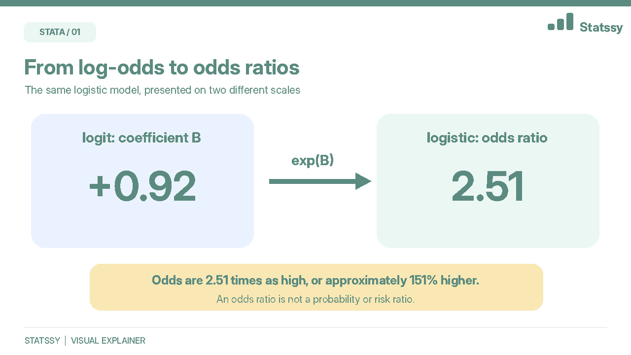
What students write: “The internship coefficient is 0.92, so the odds are 0.92 times higher.”
Why it fails: The logit coefficient is on the log-odds scale. It must be exponentiated first.
Stata fix: Run logit employed i.internship gpa, or, or check with display exp(0.92), which gives 2.51.
Correct wording: “Graduates with an internship had 2.51 times the odds of being employed, holding GPA constant.”
2. Reading odds ratios as risk ratios
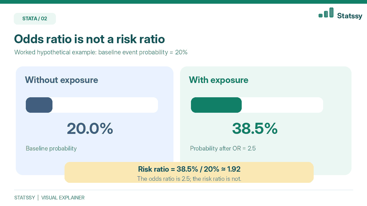
What students write: “Graduates with an internship were 2.5 times more likely to be employed.”
Why it fails: An odds ratio compares odds, not probabilities. Norton, Dowd and Maciejewski explain in JAMA that odds ratios approximate risk ratios only for rare outcomes, and the gap grows once baseline prevalence passes about 10%. They show that one odds ratio of 2.0 can mean 1% against 0.5%, or 50% against 33%, or 80% against 67%.
Case snapshot (composite example, details changed): An MBA student reported “three times more likely to quit” for an odds ratio of 3.1. The baseline quit rate was 35%. Converting to odds, multiplying by 3.1 and converting back gives about 63%, which is 1.8 times the risk, not 3.
Stata fix: Report odds, then add predicted probabilities with margins (mistake 12).
Correct wording: “Graduates with an internship had 2.51 times the odds of employment. For illustration, if the probability without an internship were 52% at a given GPA, the odds ratio would imply approximately 73% with an internship at that same GPA.” These percentages are hypothetical, not observed margins output.
I agree with the JAMA warning, but I do not ban odds ratios. Supervisors and journals still expect them. I ask students to report the odds ratio and add one probability sentence.
3. Getting odds ratios below 1 backwards
What students write: “OR = 0.60, so graduates are 60% less likely to be employed.”
Why it fails: The change in odds is (OR minus 1) times 100. So 0.60 means 40% lower odds, and “likely” is the wrong word.
Stata fix: display (0.60 - 1)*100 returns -40.
Correct wording: “Each additional year of age was associated with 40% lower odds of being employed.”
4. Ignoring confidence intervals
What students write: “GPA is significant (p = 0.026), so it clearly matters.”
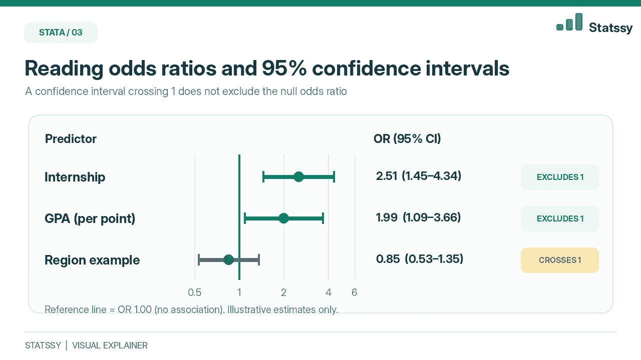
Why it fails: In my worked example below, the GPA odds ratio is 1.99 with a 95% CI from 1.09 to 3.66. The true effect could be small or large. If the interval includes 1, the result is not significant at the 5% level, as the UCLA example above shows.
Stata fix: Stata reports 95% intervals by default. Add level(99) for another level.
Correct wording: “Each one-point rise in GPA was associated with 1.99 times the odds of employment (OR = 1.99, 95% CI [1.09, 3.66]). The wide interval means the size of the effect is uncertain.”
My post on reporting effect sizes and confidence intervals covers this in more detail.
5. Using the wrong reference category
What students write: “Region 2 had higher odds.” Higher than what?
Why it fails: With i.region, Stata normally uses the lowest-coded value as the base unless you have set a different base category. If 1 means “Other” and is the base, the regional odds ratios compare against “Other”.
Stata fix: logit employed i.internship gpa ib3.region, or makes category 3 the base. Add baselevels to print the base category in the table.
Correct wording: “Compared with graduates from the North region (reference), graduates from the South had [OR] times the odds of being employed.”
6. Coding the outcome wrongly
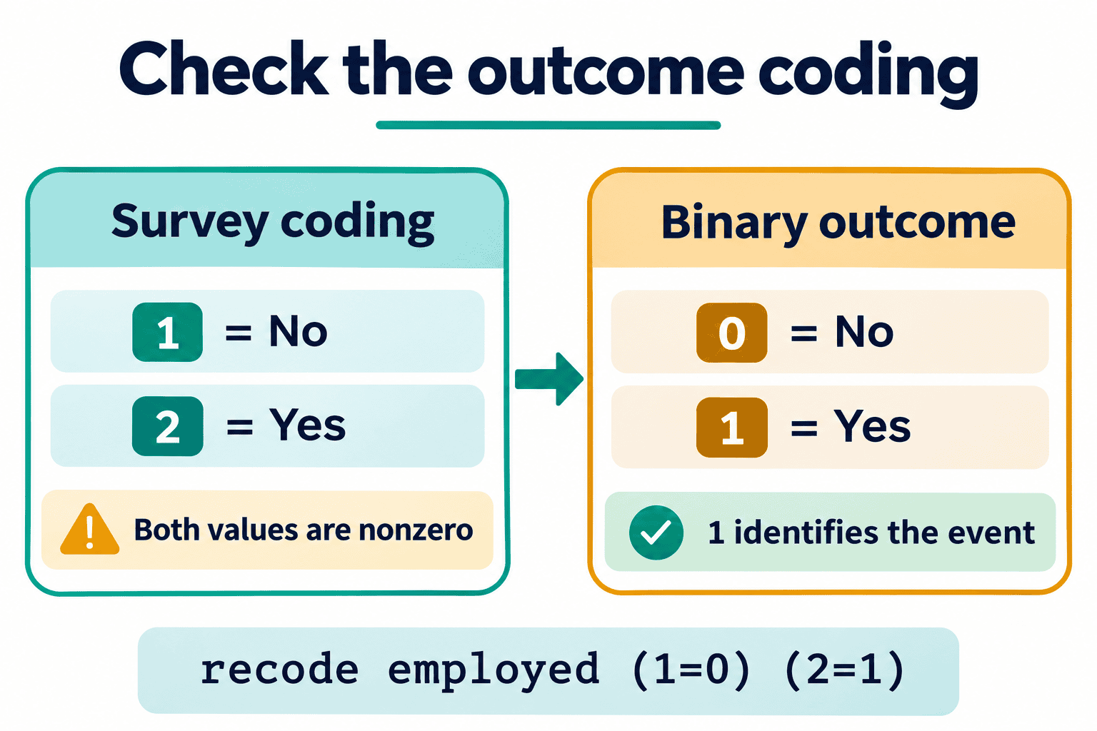
What students write: They run logit on a variable coded 1 = No and 2 = Yes.
Why it fails: Stata treats 0 as the negative outcome and every other non-missing value as positive. The UCLA seminar stresses that the outcome should be coded 0 and 1. With 1/2 coding, every case counts as positive and the model stops with an “outcome does not vary” error.
Case snapshot (composite example, details changed): A student exported survey data with 1 = No and 2 = Yes and spent two days blaming the software.
Stata fix: tab employed, then recode employed (1=0) (2=1), then label define yn 0 "No" 1 "Yes" and label values employed yn. Keep 1 for the event your sentence describes.
Correct wording: “The outcome was coded 1 if the graduate was employed within six months and 0 otherwise.”
Need help explaining an odds ratio or a regression warning?
Get guidance on how to interpret your Stata results without confusing odds, probabilities or model diagnostics.
7. Misreading odds ratios for continuous predictors
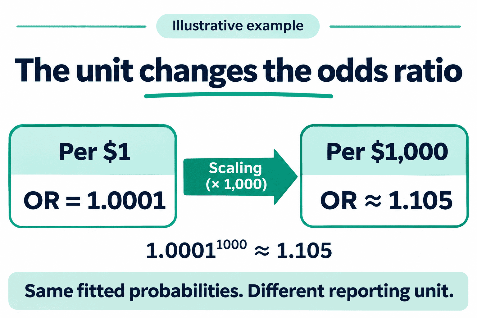
What students write: “Income has an OR of 1.0001, so it has no effect.”
Why it fails: The odds ratio is per one-unit change. If income is in pounds or dollars, one unit is tiny.
Stata fix: Rescale with gen income_k = income/1000, or standardise with egen z_income = std(income). My guide on data transformation and scaling in Stata shows when to use each.
Correct wording: “Each additional £1,000 (or $1,000) of annual income was associated with [OR] times the odds of employment.”
8. Confusing statistical with practical significance
What students write: “OR = 1.02, p < 0.001, so income strongly predicts employment.”
Why it fails: With 50,000 respondents, tiny effects become significant. An odds ratio of 1.02 per unit may change the real probability very little.
Stata fix: margins, at(income_k=(20 40 60)) shows how the predicted probability moves across income levels.
Correct wording: “Although statistically significant, the effect was small: moving from £20,000 to £60,000 raised the predicted probability of employment by about [x] percentage points.”
9. Misreading the constant and pseudo R-squared
What students write: “The constant is 0.10, so there is a 10% chance of employment. Pseudo R² is 0.04, so the model explains 4% of the variance.”
Why it fails: After logistic, _cons is the baseline odds when every predictor equals zero. That is odds, not a probability. With a continuous predictor like GPA, zero lies outside the data, so I do not interpret the constant at all. McFadden’s pseudo R² compares log-likelihoods and is not variance explained.
Hailpern and Visintainer’s Stata Journal article is the best short explanation I know of this. It warns that with interval-scaled variables in the model there is no valid reference group for the constant, and that in case-control designs the constant cannot be interpreted at all. Its main running example comes from a neonatal study and its output looks like old Stata 8 screens, so business and education students must translate it. The warning itself still holds.
Stata fix: Report the LR chi-square and its p-value. Use estat gof, group(10) as one calibration check and lroc to examine discrimination; estat classification summarises classification at a chosen cutoff. If you need odds at a meaningful value, use lincom _cons + 3*gpa, or, which gives the odds for a graduate without an internship and a GPA of 3.0.
Correct wording: “The model was significantly better than a model with no predictors (LR χ²(2) = 21.84, p < .001; McFadden pseudo R² = .04). The constant is not interpreted because a GPA of zero lies outside the observed range.”
10. Skipping assumptions, or checking the wrong ones
What students write: “Residuals were normal, so assumptions were met.”
Why it fails: Normality and constant variance belong to linear regression. Logistic regression has its own checks, listed in the next section.
Stata fix: Check linearity of the logit, multicollinearity and influential cases.
Correct wording: “Multicollinearity was checked using variance inflation factors (all below [x]), and linearity of the logit for GPA was checked with a Box-Tidwell term (p = [x]).”
11. Ignoring dropped observations and separation
What students write: “N = 412” when the dataset has 500 rows. Or an odds ratio of 4,800 described as “a very strong effect”.
Why it fails: Missing data can reduce the estimation sample without an obvious error message. See 12 Stata missing-values mistakes and how to avoid them before assuming all 500 records entered your model. Stata also flags perfect prediction with a note and may omit a predictor or observations. But near-perfect patterns, or separation spread across several variables, can slip through as huge odds ratios with enormous intervals.
Case snapshot (composite example, details changed): A student reported an odds ratio of 4,800 for a rare category where almost every graduate was employed. The confidence interval ran into the hundreds of thousands, and the student read the size as strength.
Stata fix: Run display e(N) after every model and count if e(sample)==0 to see how many observations were excluded from the estimation sample. Inspect the variables and Stata notes to determine whether missing values, perfect prediction or other restrictions caused the exclusions. For separation, collapse sparse categories, or use Firth regression: ssc install firthlogit. It is a user-written command, and its help file, as reproduced in Richard Williams’ rare-events handout, recommends likelihood-ratio tests and profile-likelihood intervals instead of Wald-based ones. See also the firthlogit package page.
My post on huge odds ratios in logistic regression is written for SPSS, but the logic is the same in Stata.
Correct wording: “Of 500 respondents, 412 had complete data and were included. Cases with missing values were excluded listwise.”
12. Stopping at odds ratios and never using margins
What students write: A table of odds ratios and nothing else.
Why it fails: Readers cannot feel odds. Predicted probabilities show what the model means in real terms.
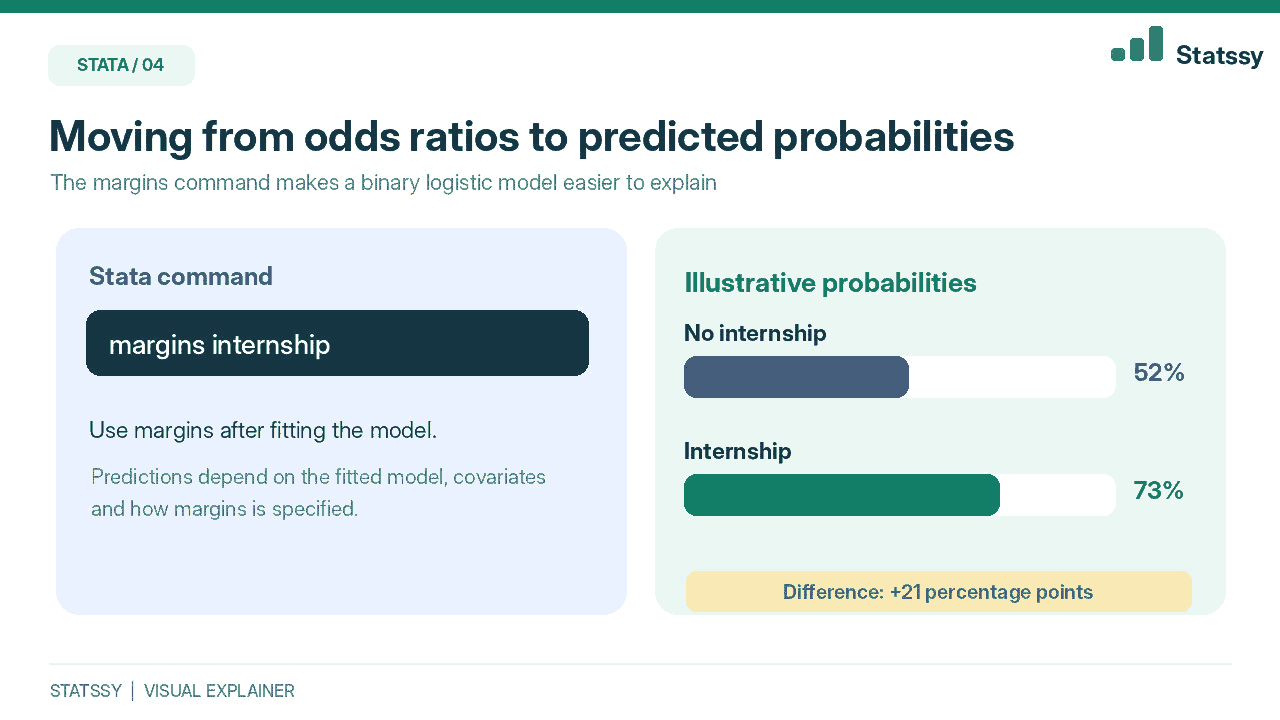
Stata fix: margins internship gives predicted probabilities. margins, dydx(*) gives average marginal effects.
Correct wording (example only): “The predicted probability of employment was 73% for graduates with an internship and 52% for those without.” Use this sentence only when your own margins output supports those values.
Good Stata logistic regression interpretation needs both the odds ratio and the probability. Luca Uberti’s 2022 Stata Journal article opens by saying the applied literature is full of interpretive and computational mistakes, and I agree. Judging by its abstract, it then offers a menu: marginal effects, partial effects, predictive margins, elasticities, and odds and risk ratios.
That menu helps a researcher but overwhelms a student with one week left. My rule is simple: odds ratios in the table, one predicted-probability sentence in the text. The abstract also argues that interaction terms are easier to interpret in practice than recent literature suggests, which is good news if your supervisor wants them.
Stata Logistic Regression Assumptions: A Quick Checklist
Binary logistic regression needs a binary outcome, independent observations, a linear relationship between continuous predictors and the log-odds, no severe multicollinearity, no highly influential cases, and enough events per predictor. It does not need normal residuals or constant variance.
| Assumption | Stata check |
|---|---|
| Binary 0/1 outcome | tab employed |
| Independent observations | Study design. For clustered data use logit ..., vce(cluster id) |
| Linear logit for continuous predictors | Box-Tidwell: gen gpa_lngpa = gpa*ln(gpa) (GPA must be above zero), add it to the model and check its p-value, or use the user-written boxtid |
| No severe multicollinearity | regress with the same variables, then estat vif (see my VIF guide) |
| No influential cases | predict dbeta, dbeta and inspect large values |
| Enough events and non-events | Check outcome frequency, number of parameters and sparse categories. The old 10-events-per-parameter rule alone is not a reliable sample-size calculation (see Riley et al., 2020). |
linktest is a useful extra, but it tests model specification, not linearity. Hailpern and Visintainer make a related point: a significant coefficient tells you nothing about whether the logit is linear. I still see students told to run normality tests on logistic models, and those tests belong to linear regression.
Stata Logistic Regression Output Interpretation: A Worked Example
This is how I present Stata logistic regression interpretation in a results chapter. The output below is illustrative, with made-up numbers from logistic employed i.internship gpa. Column labels vary slightly across Stata versions, so run it on your own data.
Logistic regression                         Number of obs   =       412
                                            LR chi2(2)      =     21.84
                                            Prob > chi2     =    0.0000
Log likelihood = -258.31                    Pseudo R2       =    0.0406

--------------------------------------------------------------------------
    employed | Odds ratio  Std. err.     z    P>|z|   [95% conf. interval]
-------------+------------------------------------------------------------
1.internship |      2.51       0.70    3.29   0.001      1.45       4.34
         gpa |      1.99       0.62    2.23   0.026      1.09       3.66
       _cons |      0.10       0.08   -2.88   0.004      0.02       0.48
--------------------------------------------------------------------------
Output note: The text table above is a constructed example, not a screenshot from a real Stata analysis. Check the command, estimates and confidence intervals against your own output before reporting results.
Read it in this order:
- N = 412. Check it matches the sample you expected.
- LR chi2 and its p-value. The model as a whole beats a model with no predictors.
- Odds ratios with confidence intervals. The GPA interval is wide, so I call that effect uncertain.
- Pseudo R2 of 0.04. This is not the percentage of variance explained and cannot, on its own, determine whether the model is useful.
_cons. I do not interpret it here, because a GPA of zero lies outside the data.
Paste-ready results paragraph
“A binary logistic regression was run to test whether internship completion and GPA predicted employment within six months. The model was statistically significant, χ²(2) = 21.84, p < .001. Graduates with an internship had 2.51 times the odds of being employed (OR = 2.51, 95% CI [1.45, 4.34], p = .001). Each one-point rise in GPA was associated with 1.99 times the odds of employment (OR = 1.99, 95% CI [1.09, 3.66], p = .026). The wide interval for GPA suggests the size of this effect should be read with caution.”
Replace every number above with your own output. These figures are illustrative and must never go into a submitted dissertation. APA 7 drops the leading zero for p (p = .026). Many UK Harvard-style departments write p = 0.026, so check your handbook.
Results table template
| Predictor | B (log-odds) | SE | OR | 95% CI | p |
|---|---|---|---|---|---|
| Internship (ref: no internship) | 0.92 | 0.28 | 2.51 | [1.45, 4.34] | .001 |
| GPA (per point) | 0.69 | 0.31 | 1.99 | [1.09, 3.66] | .026 |
| Constant | -2.30 | 0.80 | 0.10 | [0.02, 0.48] | .004 |
Note. N = 412; LR χ²(2) = 21.84, p < .001; McFadden R² = .04. The constant is shown for completeness and is not interpreted. All values are illustrative: replace them with your own output.
Interpreting Odds Ratios in Stata: Three Sentence Templates
To interpret an odds ratio, say how many times the odds change against the reference group or per one-unit increase. Hold the other variables constant, and say “odds”, not “likely”.
- Binary predictor: “Graduates with an internship had [OR] times the odds of being employed compared with those without, holding other variables constant.”
- Categorical predictor: “Compared with the North region (reference), graduates from the South had [OR] times the odds of being employed.”
- Continuous predictor: “Each one-unit increase in GPA was associated with [OR] times the odds of being employed.”
If the odds ratio is below 1, convert it to percentage lower odds, as in mistake 3.
After the Basics: Model Fit, Survey Weights and Interactions in Stata
Supervisors often ask one more question after the basics. Here are the five I hear most.
- Hosmer-Lemeshow test:
estat gof, group(10). A p-value above .05 gives no evidence of poor fit, but the test has low power in small samples and flags trivial misfit in large ones. I never rely on it alone. See Hosmer, Lemeshow and Sturdivant, Applied Logistic Regression (Wiley, 2013). - ROC and AUC:
lrocreports the area under the curve. An AUC of 0.5 means no discrimination. Hosmer, Lemeshow and Sturdivant (2013, p. 177) call 0.7 to 0.8 acceptable, 0.8 to 0.9 excellent and above 0.9 outstanding. Treat these bands as rough guides, not pass marks. - Survey weights: Declare the design with
svyset, then runsvy: logit employed i.internship gpa, or. - Interactions:
logit employed i.internship##c.gpa, or, thenmargins internship, at(gpa=(2 3 4)). Never interpret the main effects alone. - Comparing odds ratios across models: Norton and colleagues warn that odds ratios from models with different covariates are not directly comparable. On Statalist, Richard Williams of Notre Dame said that in his experience such comparisons usually produce only mildly wrong conclusions. I treat it as a caution: comment on it, and do not rank effect sizes across nested models without saying so.
For observational designs, check whether the STROBE reporting checklist (EQUATOR Network) applies to your study.
My 10-Point Stata Logistic Regression Interpretation Checklist
- Is the outcome coded 0/1, and do I know which value is the event?
- Did I state whether I report log-odds or odds ratios?
- Is every odds ratio paired with a 95% CI?
- Did I name every reference category?
- Did I say “odds”, not “likely” or “chance”?
- Are continuous predictors on a sensible scale?
- Did I check
e(N)for dropped observations? - Did I check for separation and huge odds ratios?
- Did I test the right assumptions and skip the wrong ones?
- Did I add predicted probabilities for the key results?
Keep this checklist alongside your Stata output. For a personalised explanation of a confusing odds ratio, missing-data warning or model diagnostic, use the WhatsApp contact below.
When to Get a Second Pair of Eyes on Your Results
If your odds ratios look odd, your N dropped, or your supervisor keeps writing “unclear interpretation”, get the output checked before you submit. A review now takes far less time than a resubmission.
A review explains and checks your results. The analysis and the dissertation remain your own work, so please follow your university’s policy on external help.
Not sure if you need help? Read how to know if you need a dissertation expert. If your Stata logistic regression interpretation still feels shaky, you can share what is confusing you in a WhatsApp message using the link below.
Want your results interpretation checked before submission?
Get guidance on how to interpret your Stata results without confusing odds, probabilities or model diagnostics.
FAQs
What is the difference between logit and logistic in Stata?
They fit the same model. logit shows coefficients in log-odds, while logistic shows odds ratios by default. The estimates are equivalent.
How do I get odds ratios after logit in Stata?
Add the or option, for example logit employed i.internship gpa, or. You can also run logistic instead.
Is an odds ratio the same as a risk ratio?
No. An odds ratio compares odds, and it approximates a risk ratio only when the outcome is rare. When the baseline risk is above about 10%, “times more likely” overstates the effect.
What does an odds ratio less than 1 mean?
It means lower odds of the outcome. An odds ratio of 0.60 means 40% lower odds, not “60% less likely”.
What does pseudo R-squared mean in Stata logit output?
It is McFadden’s measure of improvement over a model with no predictors. It is not variance explained, and low values are common.
How do I get predicted probabilities after logit in Stata?
Use margins, for example margins internship for predicted probabilities or margins, dydx(*) for average marginal effects. These are easier to explain than odds ratios.
What sample size do I need for logistic regression?
The old 10-events-per-parameter rule is not enough to determine sample size. Consider the number of model parameters, the frequencies of events and non-events, outcome prevalence and the precision you need. Sparse categories and rare outcomes require particular care.
How do I write logistic regression results in a dissertation?
State the model, the overall test, then each odds ratio with its 95% CI and p-value. Name the reference group and say “odds”, as in the templates above.
Should I use logit or probit in Stata?
Both give similar predicted probabilities. Logit gives odds ratios, which most supervisors expect, while probit coefficients have no odds-ratio reading.
Sources Referenced for This Stata Logistic Regression Interpretation Guide
- StataCorp manual entries for
logitandlogistic - William Gould, Interpreting logistic regression in all its forms (Stata Technical Bulletin, 2000)
- UCLA OARC, odds ratio FAQ and Stata logistic seminar
- Hailpern and Visintainer, Odds ratios and logistic regression: further examples of their use and interpretation (Stata Journal, 2003)
- Uberti, Interpreting logit models (Stata Journal, 2022)
- Norton, Dowd and Maciejewski, Odds Ratios: Current Best Practice and Use (JAMA, 2018)
- Richard Williams, Analyzing Rare Events with Logistic Regression (Notre Dame handout, reproducing the
firthlogithelp text) - Hosmer, Lemeshow and Sturdivant, Applied Logistic Regression, 3rd edition (Wiley, 2013)
About the author: I am Siddharth Gupta, an independent data consultant with more than a decade of dissertation and research support. I hold an MBA (Finance) and a BE in Electronics and Communication Engineering, and I work with Stata, R, SPSS and Power BI across marketing, finance, HR and operations. I regularly help students with Stata logistic regression interpretation. Connect with me on LinkedIn.