Why 91% Agreement Still Produced a “Poor” Score for Inter-Rater Reliability in SPSS

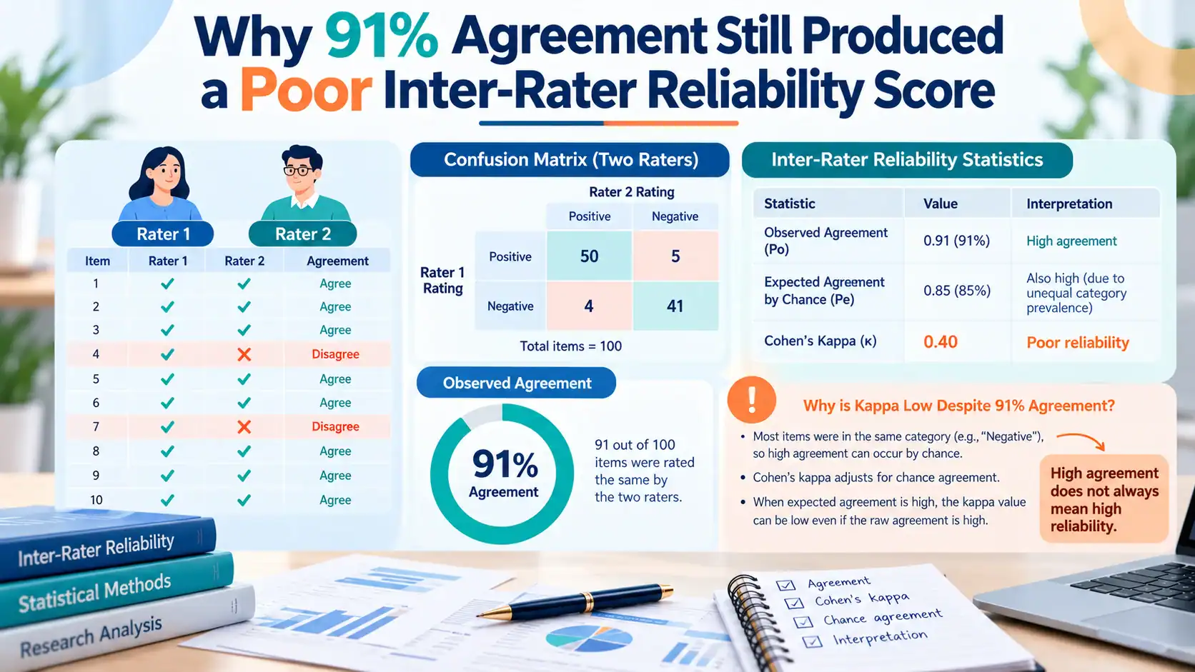
Inter-rater reliability in SPSS can show 91% raw agreement and still return a “poor” Cohen’s Kappa. Kappa corrects for chance agreement, and that correction misfires when one category dominates the data, a known issue called the kappa paradox. The fix is to report percentage agreement, PABAK, and Gwet’s AC1 alongside Kappa, not instead of it.

I watched this exact pattern nearly wreck a dissertation defence a few months ago.

A PsyD student from the School of Professional Psychology at Wright State University wrote to me about a month before her defence. She had validated a structured suicide risk assessment. Two trained raters had independently coded 120 de-identified clinical vignettes into three risk categories: low, moderate, and high.

She ran Cohen’s Kappa in SPSS on the categorical codes. The output read Kappa = .31. By most published scales that is “fair” at best, “poor” by others. She was about to write a chapter recommending against her own instrument.

Before she did that, she sent me the crosstabulation. Within an hour I could see what had actually gone wrong. It was not the instrument. It was the statistic.

91% Agreement, .31 Kappa: What Is Actually Happening

The first thing I checked was the raw crosstabulation of Rater A against Rater B. Out of 120 vignettes, the raters agreed on 109. That is 91% raw agreement, and every single disagreement was between adjacent categories, low versus moderate, or moderate versus high. Nobody swung from “low” to “high.”

Definition: The kappa paradox happens when two raters agree on the large majority of cases, yet Cohen’s Kappa still returns a low or “poor” score. This happens because a heavily skewed category distribution inflates how much agreement the correction expects by chance.

91% agreement and a Kappa of .31 sound like they cannot both be true. They can, and this exact mismatch caught an experienced student off guard a month before her defence.

What Percentage Agreement Actually Measures

Percentage agreement is the simplest reliability number there is. You count how many cases both raters coded the same way, divide by the total, done. It tells you nothing about whether that agreement could have happened purely by chance.

What Cohen’s Kappa Corrects For, and Where It Breaks

Cohen’s Kappa interpretation always starts with one formula:

κ = (Po − Pe) / (1 − Pe)

Po is observed agreement. Pe is the agreement you would expect from two raters guessing randomly, based on how often each category gets used. Kappa subtracts out the guesswork.

That correction is the whole point of Kappa, and it is a sound idea in principle. The trouble shows up when one category dominates the data. If almost every vignette gets coded “low risk,” two raters who are barely paying attention will still agree with each other most of the time purely by chance.

Kappa treats that inflated chance agreement as ground truth, and shrinks the “real” agreement to compensate. Under heavy skew, the correction can overcorrect badly enough to call a genuinely reliable instrument “poor.”

The Kappa Paradox, With the Actual Numbers

I want to show the arithmetic, because reading “high agreement, low Kappa” and actually watching the correction eat the number are two different experiences.

Here is the crosstabulation I rebuilt from the student’s data:

	Rater B: Low	Rater B: Moderate	Rater B: High	Row Total
Rater A: Low	107	5	0	112
Rater A: Moderate	4	1	1	6
Rater A: High	0	1	1	2
Column Total	111	7	2	120

93.3% of Rater A’s codes and 92.5% of Rater B’s codes fell into “low risk.” That is a far heavier skew than the general clinical vignette literature would predict, and it is exactly the condition under which the Kappa correction misfires.

Observed agreement: Po = 109 / 120 = 0.91

Expected chance agreement: Pe = (112×111 + 6×7 + 2×2) / 120² = 12,478 / 14,400 = 0.87

Kappa: κ = (0.91 − 0.87) / (1 − 0.87) = 0.04 / 0.13 = 0.31

There is your .31. Not a data entry error, not careless raters. A statistic doing precisely what it was built to do, under a marginal distribution it was never well suited to.

Feinstein and Cicchetti described this in 1990. In twelve years of untangling dissertation statistics, I still think their paper gets treated as a footnote rather than a warning label. Every methods textbook teaches the Kappa formula. Very few teach the condition under which it stops being trustworthy on its own.

Three Numbers to Report Instead of Kappa Alone

I did not tell the student to throw Kappa away. I told her to stop reporting it by itself.

1. Percentage agreement (91% here) alongside Kappa. When the two disagree by a wide margin, that gap is itself information. It tells the reader the marginals are skewed, and it stops a reviewer from reading “poor Kappa” as “unreliable instrument.”
2. PABAK (Prevalence-Adjusted Bias-Adjusted Kappa). Byrt, Bishop and Carlin proposed this in 1993 specifically for this problem, and the formula is refreshingly simple: PABAK = 2 × Po − 1 For this data, PABAK = 2 × 0.91 − 1 = 0.82, which lands in “almost perfect” territory. I like PABAK because it is transparent about what it does: it assumes the marginals should be balanced and corrects as if they were. That assumption is also its weakness. If your raters genuinely use categories at very different natural rates, PABAK can flatter the agreement more than it should. Report it alongside the raw numbers, not in place of them.
3. Gwet’s AC1. This is the newer, and to my mind the more defensible, fix. Gwet argues that Kappa’s chance model, two raters randomly guessing off the observed marginals, is not how real disagreement actually behaves. AC1 uses a different chance correction that holds up better under skew. For the same data it works out to roughly 0.90, closer to the raw agreement figure than either Kappa or PABAK.

Here is how the four numbers stack up side by side:

Statistic	Formula	Value Here	What It Tells You
Percentage Agreement	Agreements ÷ Total	91%	Raw agreement, no chance correction
Cohen’s Kappa	(Po − Pe) / (1 − Pe)	0.31	Chance-corrected, distorted by skewed marginals
PABAK	2 × Po − 1	0.82	Chance-corrected, assumes balanced marginals
Gwet’s AC1	See Gwet, 2008	~0.90	Chance-corrected, stable under skew

SPSS’s menus do not compute either of the last two for you. For PABAK and Gwet’s AC1 calculation, you are looking at manual arithmetic or R’s irrCAC package, alongside the Cohen’s Kappa Calculator for the raw figure.

One statistic I did not reach for here is weighted kappa. It softens the penalty for a “low vs moderate” disagreement compared to a “low vs high” one. Every mismatch in this data happened to be between adjacent categories, exactly the pattern weighted kappa is built to handle.

That is a genuinely useful correction, but it solves a different problem. Weighted kappa still runs through the same chance-correction machinery that caused the paradox in the first place. On data this skewed, it will not rescue Kappa on its own.

I would reach for weighted kappa on a dataset where disagreements varied more in severity, alongside PABAK and AC1, not instead of them.

It is also worth being clear about what Kappa is not. Cronbach’s alpha measures internal consistency across items on a scale, not agreement between raters. Students confuse the two often enough that I now ask which one someone means before opening SPSS.

Report all four numbers together, percentage agreement, Kappa, PABAK, and AC1, and you have given your committee a complete, honest picture instead of one number that happens to look bad.

I know the next worry: will a committee accept numbers most reviewers have never seen. In my experience, yes, provided you show your working. Cite the original papers, and present Kappa first so nobody thinks you are hiding an unflattering number. Then layer PABAK and AC1 on top as a transparency check rather than a replacement.

APA style does not mandate any single reliability statistic. It expects you to justify the one you report. A paradox you have explained in the text is far easier to defend than one a committee member spots on their own.

Inter-Rater Reliability in SPSS: Choosing the Right ICC Model

Knowing how to choose ICC model in SPSS matters as much as running the test correctly, and this is where the same student hit her second problem.

She had also run an Intraclass Correlation Coefficient on the continuous severity ratings, a 0 to 100 scale. In SPSS she had gone to Analyze, Scale, Reliability Analysis, and picked Two-Way Mixed with Absolute Agreement. That is SPSS’s default, and it is also the wrong choice more often than people realise.

SPSS offers three models, and each answers a different question:

1. One-Way Random. Use this only when different raters rated different subjects. Rare in dissertation coding work.
2. Two-Way Random. Use this when the same raters rated every subject, and you want your reliability finding to generalise beyond these two specific raters to a wider population of possible raters.
3. Two-Way Mixed. Use this when the same raters rated every subject, and you only care about the reliability of these exact two raters, nobody else.

Then comes a second choice: Consistency, which checks whether ratings move together, or Absolute Agreement, which checks whether the ratings are numerically identical. If one rater scores everyone 4 points higher, Consistency will not penalise that. Absolute Agreement will.

Her dissertation was validating an instrument for future clinical use, which means the reliability finding needed to generalise beyond her two specific raters. That called for Two-Way Random, not Two-Way Mixed.

Switching the model changed her numbers:

• Two-Way Mixed, Absolute Agreement (original): ICC = .54
• Two-Way Random, Absolute Agreement (corrected): ICC = .58
• Two-Way Random, Consistency: ICC = .71

By Koo and Li’s widely used benchmark, anything below .50 is poor, .50 to .75 is moderate, .75 to .90 is good, and .90 and above is excellent. That puts even the corrected Absolute Agreement figure at the low end of moderate, one more reason the rater gap below was worth reporting rather than glossing over.

The Consistency figure is higher because it ignores the fact that one rater scored, on average, 4.2 points higher than the other (SD = 6.1). That is a real, reportable finding, not something to bury. A Bland-Altman plot of the two raters’ scores confirmed the gap held steady across the full severity range, with no drift at the high or low end.

I had her report the Consistency ICC, the Absolute Agreement ICC, the mean rater difference, and the Bland-Altman result together, instead of one ICC number sitting alone in a table.

The Hidden Error: Training Data Mixed Into the Study Data

While going through her file I noticed something the reliability analysis had not accounted for. Before coding the 120 study vignettes, the two raters had practised on 40 separate training vignettes, discussing disagreements as they went.

Those 40 training cases were still sitting inside her reliability dataset.

That inflates every number in this article. Raters converge during training precisely because they are receiving feedback on their disagreements. Counting that convergence as part of your reliability estimate measures the training process, not the instrument itself.

Once we excluded the training vignettes and reran everything on the 120 study cases only:

• Percentage agreement: 89%
• Kappa: .28
• PABAK: .78
• AC1: .76
• ICC (Two-Way Random, Absolute Agreement): .53

Slightly lower across the board, and also the honest number. I would rather a student defend a “moderate to substantial” instrument built on clean data than a marginally better looking one built on contaminated data.

What Changed in the Dissertation

The reliability chapter went from one sentence, “Kappa = .31, indicating poor reliability,” to a full page that:

• reported percentage agreement, Kappa, PABAK, and Gwet’s AC1 side by side
• named the kappa paradox explicitly and showed the marginal distributions
• corrected the ICC model from Two-Way Mixed to Two-Way Random, with a stated reason
• reported both the Consistency and Absolute Agreement ICCs
• added a Bland-Altman analysis for the rater gap
• excluded the training vignettes from the final numbers
• described the instrument as showing moderate to substantial reliability, not poor reliability

The committee accepted the revision, and her defence went ahead on schedule. That outcome is the whole reason inter-rater reliability in SPSS deserves more attention than a single output line, since one misread statistic nearly cost her the chapter.

If your instrument is a validated scale rather than a custom instrument, you are less likely to run into this particular mess. Published scales are usually piloted on samples where category balance has already been checked. Building your own coding scheme, the way this student did, means you inherit the responsibility of checking that balance yourself. It also helps to know whether you are working with single-item or multi-item measures, since that changes which reliability statistic applies in the first place.

FAQ

If you are looking for statistics help for PsyD dissertation research, start by checking your marginal distribution before you trust a single Kappa value on sight. If a statistic like this one has you second-guessing your whole reliability chapter, that is usually a sign it is worth checking whether you actually need outside help before you write the conclusion.

I have seen this exact pattern often enough in statistical consulting work for dissertations over twelve years that it is usually the first thing I check now. Raw data stays confidential and de-identified, and a reliability check like this one is typically a same-week turnaround, not a multi-week engagement. If this is your first time running these tests under deadline pressure, an SPSS reliability walkthrough with a tutor is worth the hour it takes.

Siddharth Gupta

I have spent twelve years as an independent statistics consultant, holding an MBA in Finance and an M.Tech, working across R, SPSS, and Stata for dissertation and thesis clients. Connect with me on LinkedIn.

Client and case details in this article have been changed to protect confidentiality.