Trend Analysis in R using real world data in 2024

Introduction

Recently I was searching for something interesting in Google trends and suddenly thought why not check how `ggplot` is performing. I know its random but just hit my mind and I landed up finding traffic on search term ggplot. I found the chart below and was quite astonished by its beautiful pattern.

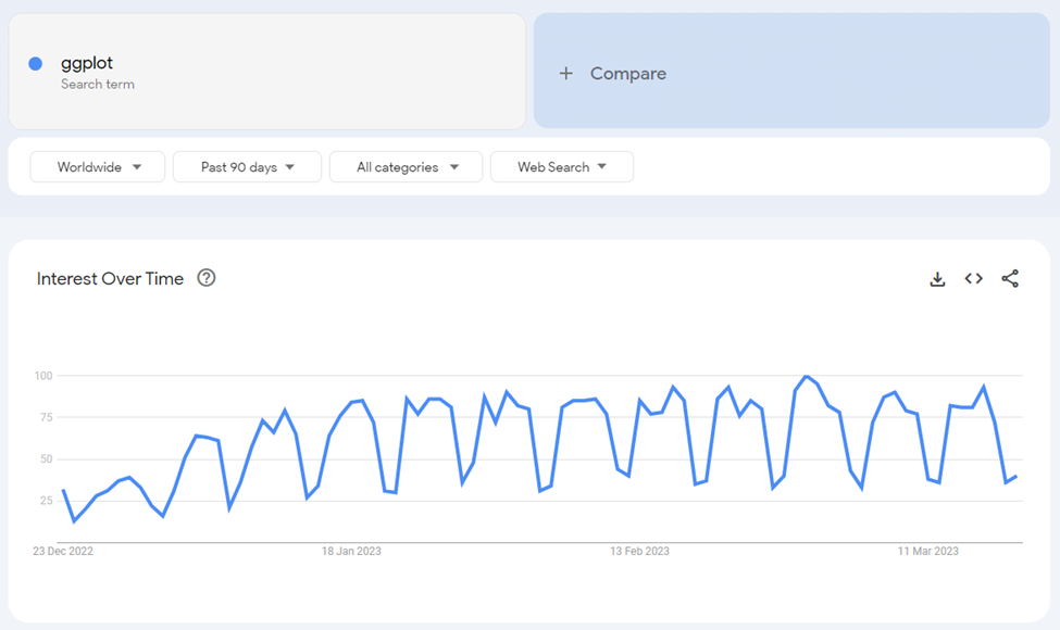
You can see this chart is both interesting and a great example to demonstrate the power of R in analysis.

So, I thought let’s analyze the trend for ggplot using R!!!!

In this article, we will learn how to find the trend and seasonality of a time series using R and will predict what will be the future of ggplot searches.Trend Analysis in R

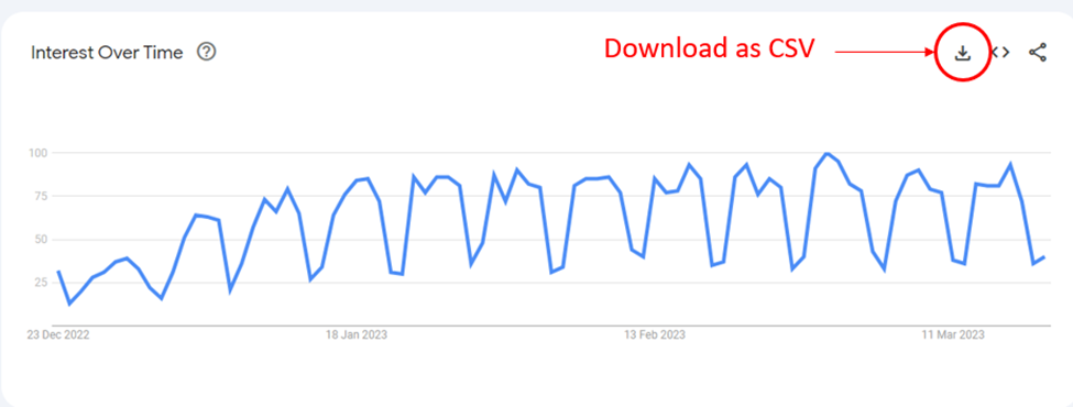
So the first step is to download this data into CSV. You can do that by clicking on the download button.

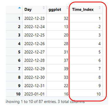
After you download the data, you will find the data looks something like this,

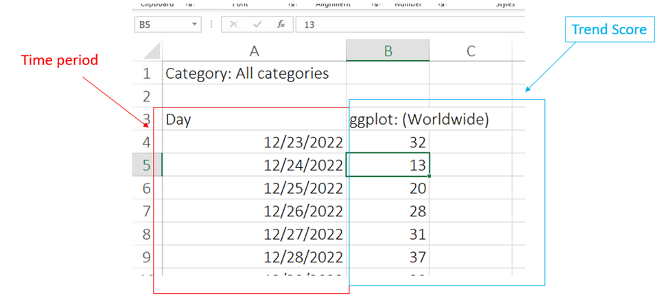
So now we have two columns, one is the day on which the data is recorded and second is the actual data which we will analyze. The first step in any analysis is “Data Cleaning”

So as a good data scientist, it is important to make sure that when we import this data to R, it do not increase our workload.Trend Analysis in R

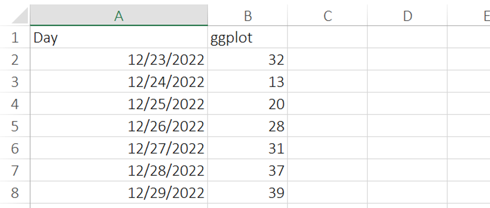
I am deleting the first two rows to ensure that my column headings i.e. “Day” and “ggplot: (Worldwide)” comes in the first row and rename it to “ggplot”. See how it will look like

Now start your R environment and import this data into R. Keep the files in the same directory to avoid confusion. Use the following commands:

library(readr)
dataset <- read_csv("multiTimeline.csv")
View(dataset)
str(dataset)  #to check the structure of data

Now, lets first convert this data into a time series data because you know it’s a time series data but R doesn’t know yet. (Why?)

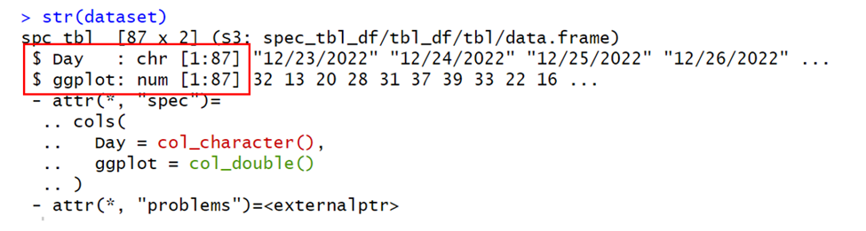
When you run the last command, you will see the structure of data and as seen, Day column is “chr” which means character. This indicates R did not understand that this is a date column. So, we need to explain it to R.

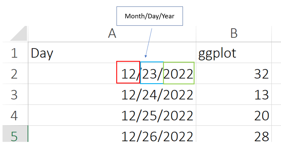
If you see that data carefully, our date is Month/Day/Year.

We will convert this to time using R and check the structure again,

dataset$Day <- as.Date(dataset$Day, "%m/%d/%Y")
str(dataset)

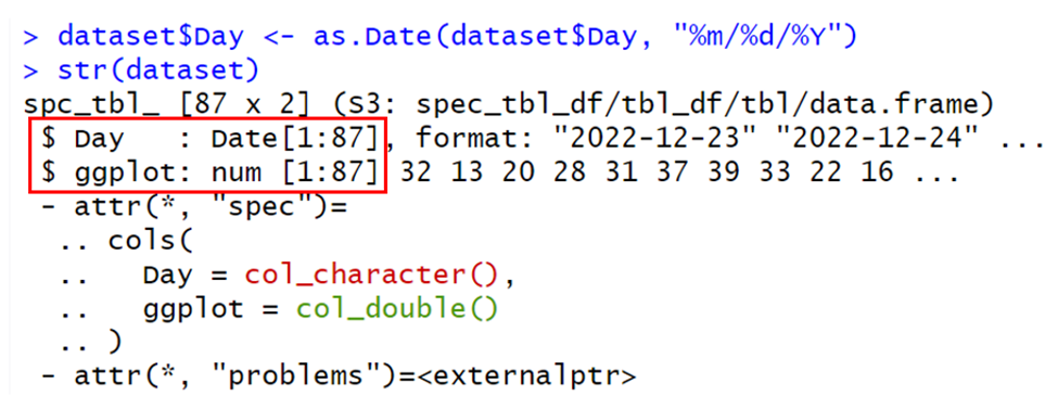
Congratulations 😊. We got day column converted to “Date” type. Now, we can easily convert our data into time series.

Now let’s visualize the same series in R using ggplot,Trend Analysis in R

# load the ggplot2 package
library(ggplot2)

# create a line plot using ggplot
ggplot(dataset, aes(x = Day, y = ggplot)) +
  geom_line() +
  labs(title = "Sales over Time", x = "Date", y = "Sales")+theme_classic()

Once you run the code above, you will find a time series chart same as below

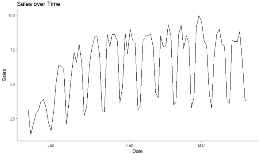
Now why is this time series interesting? Because there are two main components we can see here.

(i) Trend – Trend refers to the long-term movement or direction of a time series data. It shows whether the values are increasing or decreasing over time.

(ii) Seasonal Variations – Seasonal variations refer to the pattern that repeats itself after a fixed interval of time, such as daily, weekly, monthly, or yearly.

We can say that variations are cyclic, but since the approximate width of each cycle is similar, we will call it seasonal variations rather than cyclic variations.

But for this article we are focussing on Trend. For seasonal variations click here

Now to find the trend, we have to think of it as a straight line which either increases or decreases with time. So for our data we will create a new variable which represents time progression.

# Add a numeric time index to the data frame
dataset$Time_Index <- 1:nrow(dataset)

This will add an additional column to the dataframe with first day as 1 and so on.

Mathematically we write trend as,

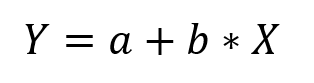
Where,

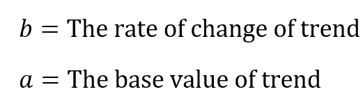
To do this in R we have to apply simple linear regression,

# Fit a linear regression model to the data to obtain the trend component
trend_model <- lm(ggplot ~ Time_Index, data = dataset)
print(trend_model)

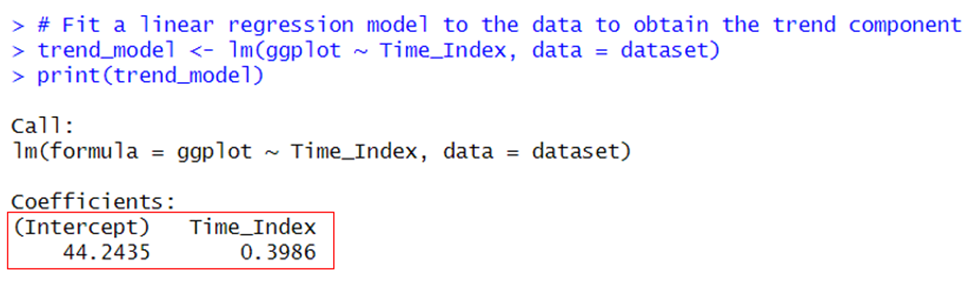
So after running the code you will find this result which shows intercept and time_index. Here the Intercept is your b and Time_Index is your a for the trend component.

So now we have value of a and b, we can write our trend component as,

So what does this show?

(i) First it shows that on the very first day in the past 90 days, the search volume score for GGPLOT was 44.24 units.

(ii) Second it shows that every day from the first day, the search volume is increase by 0.3986 units because the value is positive. This means that every next day, there will be additional 0.3986 units of search as we move forward in time.

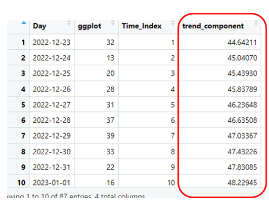
Now let’s find out what are the values of search volume that trend component suggests. We will add a new column to our dataset for this using the mathematical equation above.

# Calculating predicted search volume
dataset$trend_component <- trend_model$coefficients[1] + trend_model$coefficients[2] * dataset$Time_Index

Now lets plot it using ggplot 😊

# create a line plot using ggplot
ggplot(dataset, aes(x = Day, y = ggplot)) +
  geom_line() + geom_line(aes(y= trend_component), color = "red")+
  labs(title = "Sales over Time", x = "Date", y = "Sales")+theme_classic()

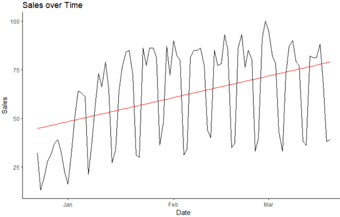
Here you will find the red colored line representing the trend and it clearly shows a positive upward moving direction. So, if you are learning ggplot, then go ahead! The requirements will increase in future.

Now, after doing this, try to understand the situation, we analyzed only past 90 days it means the condition may vary in future but as of now, we can comfortably say that searches for GGPLOT is increasing.

Trend Analysis in R using real world data in 2024